We Are Again Working With the Characters Abbs C Ma Me Mi Mo Mu
R basics
In this book, nosotros will exist using the R software surround for all our assay. You will learn R and data assay techniques simultaneously. To follow along yous will therefore need admission to R. We also recommend the employ of an integrated development environment (IDE), such equally RStudio, to save your piece of work. Note that information technology is common for a course or workshop to offer admission to an R environment and an IDE through your web browser, equally done by RStudio cloud12. If you have access to such a resources, you don't demand to install R and RStudio. However, if yous intend on condign an advanced data annotator, nosotros highly recommend installing these tools on your figurer13. Both R and RStudio are free and available online.
Case study: US Gun Murders
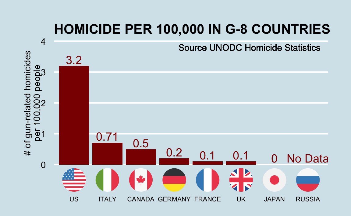
Imagine you live in Europe and are offered a chore in a US visitor with many locations beyond all states. It is a great job, but news with headlines such as Us Gun Homicide Rate College Than Other Developed Countries 14 have you worried. Charts like this may business you even more than:
Or even worse, this version from everytown.org: 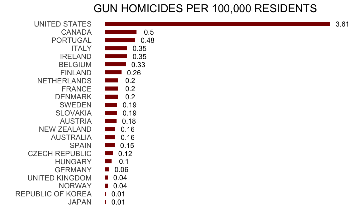
But then you remember that the Us is a large and various country with 50 very different states equally well every bit the District of Columbia (DC).
#> Warning: Information technology is deprecated to specify `guide = FALSE` to remove a guide. #> Please use `guide = "none"` instead. 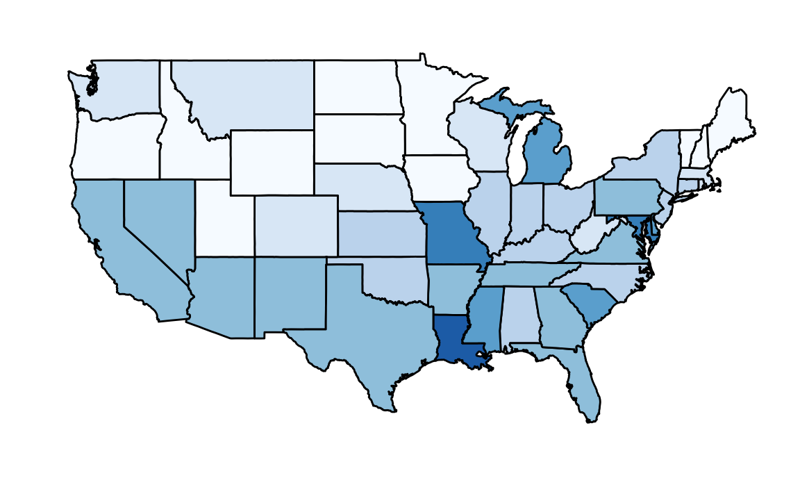
California, for example, has a larger population than Canada, and twenty US states have populations larger than that of Norway. In some respects, the variability across states in the US is akin to the variability across countries in Europe. Furthermore, although non included in the charts above, the murder rates in Lithuania, Ukraine, and Russian federation are college than 4 per 100,000. So perchance the news reports that worried you are too superficial. You have options of where to live and desire to determine the safety of each detail country. Nosotros will proceeds some insights by examining data related to gun homicides in the Usa during 2010 using R.
Before we go started with our example, we need to cover logistics as well every bit some of the very basic edifice blocks that are required to gain more advanced R skills. Be aware that the usefulness of some of these building blocks may not be immediately obvious, but afterward in the volume you will appreciate having mastered these skills.
The very basics
Before we get started with the motivating dataset, we need to cover the very nuts of R.
Objects
Suppose a high school student asks usa for help solving several quadratic equations of the class \(ax^2+bx+c = 0\). The quadratic formula gives us the solutions:
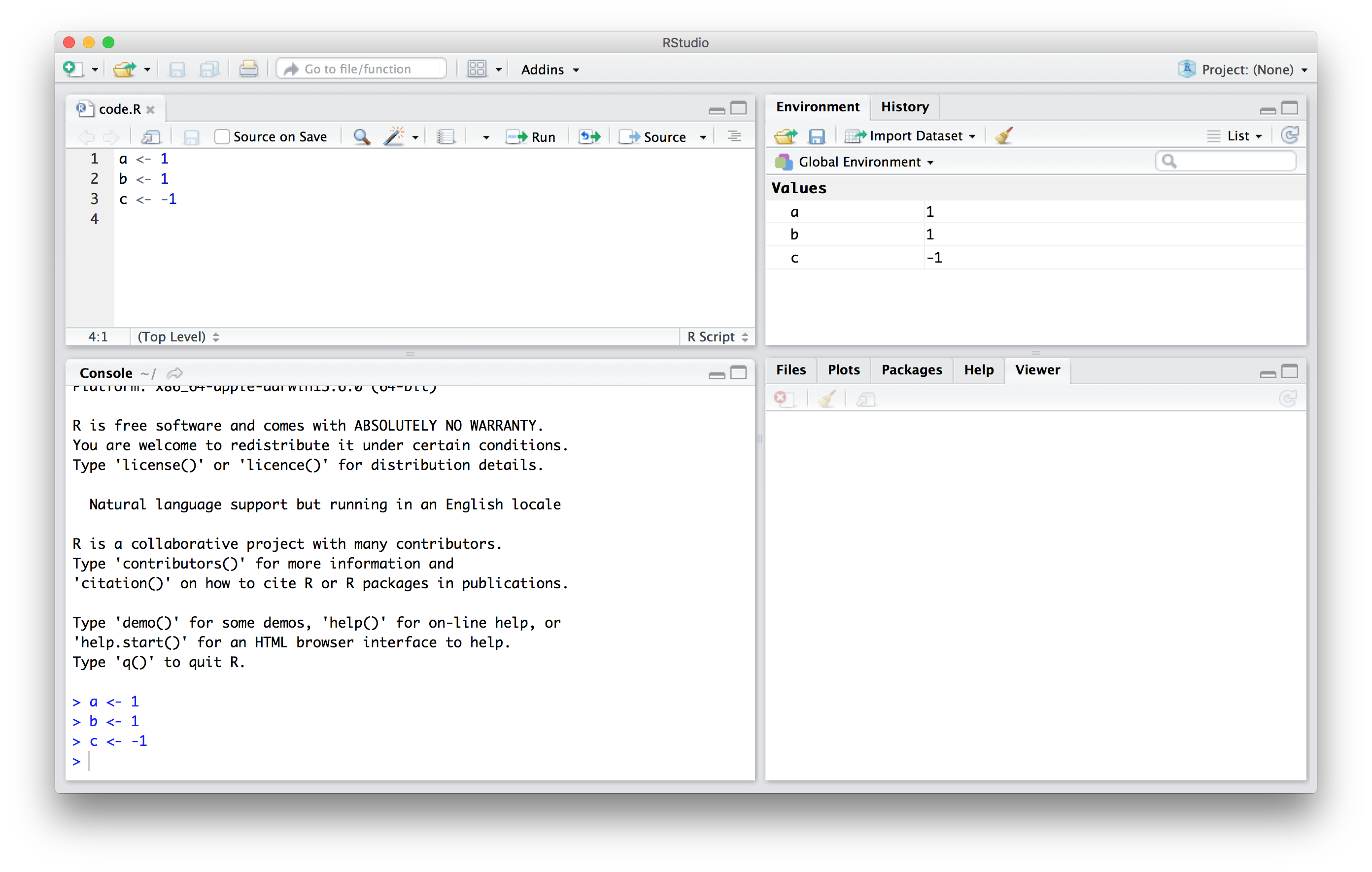
\[ \frac{-b - \sqrt{b^2 - 4ac}}{2a}\,\, \mbox{ and } \frac{-b + \sqrt{b^ii - 4ac}}{2a} \] which of class change depending on the values of \(a\), \(b\), and \(c\). Ane advantage of programming languages is that nosotros tin can ascertain variables and write expressions with these variables, similar to how nosotros exercise so in math, simply obtain a numeric solution. We volition write out general code for the quadratic equation below, merely if we are asked to solve \(x^two + x -1 = 0\), then we ascertain:
which stores the values for afterwards utilize. We use <- to assign values to the variables.
We tin can also assign values using = instead of <-, just nosotros recommend against using = to avoid defoliation.
Copy and paste the code above into your console to define the three variables. Notation that R does not print anything when nosotros make this assignment. This ways the objects were defined successfully. Had you made a mistake, yous would take received an mistake message.
To see the value stored in a variable, we simply ask R to evaluate a and it shows the stored value:
A more than explicit manner to enquire R to show u.s. the value stored in a is using print like this:
Nosotros employ the term object to draw stuff that is stored in R. Variables are examples, but objects can as well be more complicated entities such as functions, which are described subsequently.
The workspace
As we define objects in the panel, nosotros are really changing the workspace. You can encounter all the variables saved in your workspace past typing:
ls() #> [1] "a" "b" "c" "dat" "img_path" "murders" In RStudio, the Surroundings tab shows the values:
Nosotros should meet a, b, and c. If you endeavor to recover the value of a variable that is non in your workspace, y'all receive an error. For case, if you type x you will receive the following bulletin: Mistake: object 'x' not plant.
At present since these values are saved in variables, to obtain a solution to our equation, we use the quadratic formula:
(-b + sqrt(b^ two - four *a*c) ) / ( 2 *a ) #> [one] 0.618 (-b - sqrt(b^ 2 - iv *a*c) ) / ( 2 *a ) #> [1] -i.62 Functions
Once you define variables, the data analysis process can usually be described as a series of functions applied to the data. R includes several predefined functions and most of the analysis pipelines we construct brand extensive use of these.
We already used the install.packages, library, and ls functions. We also used the function sqrt to solve the quadratic equation above. There are many more prebuilt functions and even more tin be added through packages. These functions do not appear in the workspace because you lot did not define them, but they are available for immediate use.
In general, we demand to use parentheses to evaluate a function. If yous type ls, the function is not evaluated and instead R shows you lot the code that defines the function. If you type ls() the function is evaluated and, as seen above, we see objects in the workspace.
Unlike ls, virtually functions require one or more arguments. Beneath is an instance of how nosotros assign an object to the argument of the function log. Remember that we earlier defined a to exist 1:
log(8) #> [ane] two.08 log(a) #> [1] 0 You tin can observe out what the function expects and what it does by reviewing the very useful manuals included in R. You can get help by using the help function similar this:
For most functions, we can too utilise this shorthand:
The aid page will show yous what arguments the role is expecting. For example, log needs 10 and base to run. Notwithstanding, some arguments are required and others are optional. You lot can determine which arguments are optional past noting in the aid certificate that a default value is assigned with =. Defining these is optional. For example, the base of operations of the office log defaults to base = exp(one) making log the natural log by default.
If you want a quick await at the arguments without opening the help system, you can type:
args(log) #> role (ten, base = exp(1)) #> Cypher You can modify the default values by but assigning another object:
log(8, base = 2) #> [ane] 3 Note that nosotros have non been specifying the argument x every bit such:
log(10 = 8, base = 2) #> [ane] iii The above lawmaking works, merely nosotros tin save ourselves some typing: if no argument name is used, R assumes y'all are entering arguments in the order shown in the help file or past args. So by not using the names, it assumes the arguments are x followed by base of operations:
If using the arguments' names, then we can include them in whatever gild we want:
log(base = two, 10 = 8) #> [1] 3 To specify arguments, we must use =, and cannot use <-.
There are some exceptions to the rule that functions need the parentheses to be evaluated. Amongst these, the most commonly used are the arithmetic and relational operators. For example:
You can see the arithmetics operators by typing:
or
and the relational operators by typing:
or
Other prebuilt objects
There are several datasets that are included for users to practise and examination out functions. You can come across all the bachelor datasets by typing:
This shows you the object proper name for these datasets. These datasets are objects that can exist used by just typing the name. For example, if you type:
R will testify you Mauna Loa atmospheric CO2 concentration data.
Other prebuilt objects are mathematical quantities, such equally the constant \(\pi\) and \(\infty\):
pi #> [ane] 3.14 Inf + 1 #> [i] Inf Variable names
We have used the messages a, b, and c as variable names, simply variable names can exist almost anything. Some basic rules in R are that variable names accept to start with a letter of the alphabet, tin't incorporate spaces, and should not be variables that are predefined in R. For example, don't name 1 of your variables install.packages past typing something like install.packages <- ii.
A overnice convention to follow is to use meaningful words that describe what is stored, use only lower case, and utilize underscores as a substitute for spaces. For the quadratic equations, we could utilise something like this:
solution_1 <- (-b + sqrt(b^ 2 - 4 *a*c)) / (2 *a) solution_2 <- (-b - sqrt(b^ 2 - 4 *a*c)) / (2 *a) For more advice, we highly recommend studying Hadley Wickham'southward style guidexv.
Saving your workspace
Values remain in the workspace until you terminate your session or erase them with the function rm. Just workspaces besides can be saved for later utilise. In fact, when you quit R, the program asks you if you want to salve your workspace. If you do save information technology, the adjacent fourth dimension y'all start R, the programme volition restore the workspace.
We actually recommend against saving the workspace this way considering, as yous start working on different projects, it volition go harder to proceed rails of what is saved. Instead, we recommend yous assign the workspace a specific proper noun. You can practise this by using the function save or save.prototype. To load, utilize the role load. When saving a workspace, we recommend the suffix rda or RData. In RStudio, y'all tin also do this by navigating to the Session tab and choosing Relieve Workspace equally. You can later load it using the Load Workspace options in the same tab. Y'all can read the aid pages on save, save.image, and load to learn more.
Motivating scripts
To solve another equation such equally \(3x^2 + 2x -one\), we can copy and paste the code in a higher place and so redefine the variables and recompute the solution:
a <- iii b <- ii c <- - one (-b + sqrt(b^ 2 - four *a*c)) / (2 *a) (-b - sqrt(b^ 2 - iv *a*c)) / (2 *a) Past creating and saving a script with the code above, nosotros would not need to retype everything each fourth dimension and, instead, simply modify the variable names. Try writing the script higher up into an editor and find how easy it is to change the variables and receive an answer.
Exercises
1. What is the sum of the start 100 positive integers? The formula for the sum of integers \(i\) through \(n\) is \(n(northward+1)/2\). Define \(n=100\) and and so apply R to compute the sum of \(1\) through \(100\) using the formula. What is the sum?
2. At present use the same formula to compute the sum of the integers from 1 through 1,000.
3. Look at the effect of typing the post-obit lawmaking into R:
northward <- chiliad x <- seq(1, north) sum(x) Based on the issue, what do you think the functions seq and sum do? Yous can use aid.
-
sumcreates a list of numbers andseqadds them upwardly. -
seqcreates a listing of numbers andsumadds them upward. -
seqcreates a random list andsumcomputes the sum of 1 through 1,000. -
sumalways returns the same number.
4. In math and programming, we say that nosotros evaluate a office when we replace the argument with a given number. And so if we blazon sqrt(4), we evaluate the sqrt function. In R, yous can evaluate a function inside another office. The evaluations happen from the inside out. Utilise one line of code to compute the log, in base of operations x, of the square root of 100.
5. Which of the following volition always render the numeric value stored in 10? You can try out examples and use the help organization if you want.
-
log(x^x) -
log10(x^10) -
log(exp(x)) -
exp(log(x, base = 2))
Data types
Variables in R can be of unlike types. For example, we need to distinguish numbers from character strings and tables from simple lists of numbers. The office form helps united states decide what type of object we take:
a <- 2 class(a) #> [1] "numeric" To work efficiently in R, it is important to learn the dissimilar types of variables and what we can do with these.
Information frames
Up to now, the variables nosotros have defined are just one number. This is non very useful for storing information. The virtually common way of storing a dataset in R is in a information frame. Conceptually, nosotros can think of a data frame as a table with rows representing observations and the different variables reported for each observation defining the columns. Data frames are particularly useful for datasets because nosotros can combine different data types into ane object.
A big proportion of data assay challenges start with information stored in a information frame. For example, we stored the data for our motivating example in a information frame. You tin can admission this dataset by loading the dslabs library and loading the murders dataset using the data function:
library(dslabs) data(murders) To see that this is in fact a information frame, nosotros type:
class(murders) #> [1] "data.frame" Examining an object
The function str is useful for finding out more nearly the structure of an object:
str(murders) #> 'data.frame': 51 obs. of 5 variables: #> $ state : chr "Alabama" "Alaska" "Arizona" "Arkansas" ... #> $ abb : chr "AL" "AK" "AZ" "AR" ... #> $ region : Cistron westward/ four levels "Northeast","S",..: 2 four 4 2 4 4 1 two ii #> 2 ... #> $ population: num 4779736 710231 6392017 2915918 37253956 ... #> $ full : num 135 19 232 93 1257 ... This tells us much more about the object. We see that the table has 51 rows (l states plus DC) and five variables. We tin can show the first six lines using the function caput:
caput(murders) #> state abb region population total #> one Alabama AL South 4779736 135 #> 2 Alaska AK West 710231 19 #> 3 Arizona AZ West 6392017 232 #> 4 Arkansas AR Southward 2915918 93 #> v California CA West 37253956 1257 #> vi Colorado CO Westward 5029196 65 In this dataset, each land is considered an observation and 5 variables are reported for each state.
Earlier we go whatever further in answering our original question well-nigh different states, let'south learn more about the components of this object.
The accessor: $
For our analysis, we will need to access the different variables represented by columns included in this data frame. To do this, we employ the accessor operator $ in the following way:
murders$population #> [1] 4779736 710231 6392017 2915918 37253956 5029196 3574097 #> [viii] 897934 601723 19687653 9920000 1360301 1567582 12830632 #> [15] 6483802 3046355 2853118 4339367 4533372 1328361 5773552 #> [22] 6547629 9883640 5303925 2967297 5988927 989415 1826341 #> [29] 2700551 1316470 8791894 2059179 19378102 9535483 672591 #> [36] 11536504 3751351 3831074 12702379 1052567 4625364 814180 #> [43] 6346105 25145561 2763885 625741 8001024 6724540 1852994 #> [fifty] 5686986 563626 Only how did we know to use population? Previously, by applying the role str to the object murders, we revealed the names for each of the five variables stored in this table. We tin quickly access the variable names using:
names(murders) #> [ane] "state" "abb" "region" "population" "total" It is important to know that the order of the entries in murders$population preserves the order of the rows in our data tabular array. This will subsequently permit united states of america to manipulate one variable based on the results of some other. For example, we will be able to order the land names by the number of murders.
Tip: R comes with a very overnice auto-consummate functionality that saves us the trouble of typing out all the names. Try typing murders$p then hitting the tab fundamental on your keyboard. This functionality and many other useful auto-complete features are available when working in RStudio.
Vectors: numerics, characters, and logical
The object murders$population is not one number but several. Nosotros call these types of objects vectors. A single number is technically a vector of length ane, merely in general we utilize the term vectors to refer to objects with several entries. The function length tells you how many entries are in the vector:
popular <- murders$population length(pop) #> [ane] 51 This detail vector is numeric since population sizes are numbers:
class(pop) #> [1] "numeric" In a numeric vector, every entry must exist a number.
To store character strings, vectors can likewise be of class graphic symbol. For case, the land names are characters:
class(murders$country) #> [1] "character" Every bit with numeric vectors, all entries in a character vector need to exist a character.
Another of import type of vectors are logical vectors. These must exist either TRUE or FALSE.
z <- 3 == 2 z #> [1] Simulated grade(z) #> [1] "logical" Hither the == is a relational operator asking if three is equal to 2. In R, if you just use one =, you actually assign a variable, but if you utilise ii == you test for equality.
Yous tin run across the other relational operators past typing:
In time to come sections, you will run into how useful relational operators can be.
Nosotros discuss more important features of vectors after the side by side set of exercises.
Advanced: Mathematically, the values in pop are integers and there is an integer form in R. Yet, by default, numbers are assigned class numeric even when they are circular integers. For example, class(1) returns numeric. You can turn them into class integer with the as.integer() part or past calculation an 50 like this: 1L. Note the course by typing: grade(1L)
Factors
In the murders dataset, we might await the region to also be a character vector. However, it is non:
class(murders$region) #> [one] "gene" It is a gene. Factors are useful for storing chiselled information. Nosotros can see that there are only 4 regions past using the levels part:
levels(murders$region) #> [1] "Northeast" "South" "Northward Key" "West" In the background, R stores these levels as integers and keeps a map to go on track of the labels. This is more retention efficient than storing all the characters.
Note that the levels take an club that is dissimilar from the lodge of appearance in the factor object. The default in R is for the levels to follow alphabetical social club. Withal, often we want the levels to follow a unlike guild. You can specify an gild through the levels statement when creating the gene with the cistron function. For example, in the murders dataset regions are ordered from e to westward. The office reorder lets us alter the club of the levels of a gene variable based on a summary computed on a numeric vector. Nosotros volition demonstrate this with a simple case, and will see more advanced ones in the Data Visualization part of the book.
Suppose we want the levels of the region by the total number of murders rather than alphabetical order. If in that location are values associated with each level, we can utilize the reorder and specify a data summary to make up one's mind the order. The following code takes the sum of the total murders in each region, and reorders the cistron post-obit these sums.
region <- murders$region value <- murders$total region <- reorder(region, value, FUN = sum) levels(region) #> [i] "Northeast" "North Central" "West" "South" The new society is in agreement with the fact that the Northeast has the to the lowest degree murders and the South has the well-nigh.
Warning: Factors can be a source of defoliation since sometimes they acquit like characters and sometimes they exercise non. As a result, confusing factors and characters are a common source of bugs.
Lists
Information frames are a special case of lists. Lists are useful because yous can shop any combination of different types. You can create a listing using the list part like this:
record <- list(name = "John Doe", student_id = 1234, grades = c(95, 82, 91, 97, 93), final_grade = "A") The role c is described in Section 2.half-dozen.
This listing includes a character, a number, a vector with five numbers, and some other character.
record #> $name #> [i] "John Doe" #> #> $student_id #> [1] 1234 #> #> $grades #> [1] 95 82 91 97 93 #> #> $final_grade #> [1] "A" class(tape) #> [1] "list" Every bit with information frames, you lot can extract the components of a list with the accessor $.
record$student_id #> [1] 1234 We can besides use double square brackets ([[) like this:
tape[["student_id"]] #> [1] 1234 You should get used to the fact that in R, there are frequently several ways to do the aforementioned thing, such equally accessing entries.
You might besides encounter lists without variable names.
record2 <- listing("John Doe", 1234) record2 #> [[1]] #> [ane] "John Doe" #> #> [[2]] #> [1] 1234 If a list does not take names, you cannot extract the elements with $, just you tin however utilize the brackets method and instead of providing the variable name, you provide the listing index, similar this:
record2[[i]] #> [ane] "John Doe" We won't be using lists until later, just you might encounter one in your own exploration of R. For this reason, we show you some basics here.
Matrices
Matrices are another type of object that are mutual in R. Matrices are similar to data frames in that they are ii-dimensional: they have rows and columns. All the same, similar numeric, grapheme and logical vectors, entries in matrices have to be all the same type. For this reason data frames are much more than useful for storing data, since we can have characters, factors, and numbers in them.
Yet matrices have a major advantage over data frames: nosotros can perform matrix algebra operations, a powerful type of mathematical technique. We do not describe these operations in this book, but much of what happens in the groundwork when you perform a data analysis involves matrices. We embrace matrices in more than detail in Chapter 34.1 but draw them briefly here since some of the functions nosotros will acquire return matrices.
Nosotros can define a matrix using the matrix office. We demand to specify the number of rows and columns.
mat <- matrix(1 : 12, 4, 3) mat #> [,ane] [,ii] [,3] #> [1,] 1 5 9 #> [ii,] 2 6 10 #> [3,] 3 vii 11 #> [4,] 4 eight 12 You can access specific entries in a matrix using square brackets ([). If you lot want the second row, third cavalcade, y'all employ:
If y'all want the entire second row, you leave the column spot empty:
Notice that this returns a vector, not a matrix.
Similarly, if you want the unabridged 3rd column, you get out the row spot empty:
mat[, 3] #> [1] ix ten 11 12 This is also a vector, not a matrix.
Yous can access more than one column or more than one row if you like. This will give you a new matrix.
mat[, 2 : 3] #> [,1] [,2] #> [ane,] 5 9 #> [2,] 6 10 #> [iii,] seven 11 #> [iv,] 8 12 You can subset both rows and columns:
mat[ane : 2, two : 3] #> [,1] [,ii] #> [ane,] 5 9 #> [2,] 6 10 We can catechumen matrices into information frames using the role as.data.frame:
as.data.frame(mat) #> V1 V2 V3 #> ane i five 9 #> ii 2 vi 10 #> iii 3 7 11 #> four 4 8 12 You can also use single square brackets ([) to access rows and columns of a data frame:
data("murders") murders[25, 1] #> [1] "Mississippi" murders[2 : iii, ] #> state abb region population total #> two Alaska AK Due west 710231 19 #> 3 Arizona AZ West 6392017 232 Exercises
1. Load the U.s.a. murders dataset.
library(dslabs) data(murders) Employ the function str to examine the structure of the murders object. Which of the following all-time describes the variables represented in this data frame?
- The 51 states.
- The murder rates for all 50 states and DC.
- The state name, the abridgement of the state name, the state'south region, and the state's population and full number of murders for 2010.
-
strshows no relevant information.
2. What are the column names used by the data frame for these 5 variables?
3. Employ the accessor $ to extract the state abbreviations and assign them to the object a. What is the class of this object?
iv. Now employ the square brackets to extract the state abbreviations and assign them to the object b. Employ the identical function to make up one's mind if a and b are the same.
5. We saw that the region column stores a factor. You can corroborate this by typing:
With i line of lawmaking, use the role levels and length to decide the number of regions defined by this dataset.
half dozen. The function table takes a vector and returns the frequency of each element. You can rapidly run across how many states are in each region by applying this function. Use this role in one line of code to create a table of states per region.
Vectors
In R, the well-nigh bones objects available to shop information are vectors. As we take seen, complex datasets can usually be broken downward into components that are vectors. For instance, in a data frame, each column is a vector. Here we acquire more about this important class.
Creating vectors
We can create vectors using the function c, which stands for concatenate. We use c to concatenate entries in the following way:
codes <- c(380, 124, 818) codes #> [1] 380 124 818 Nosotros tin can besides create character vectors. We employ the quotes to announce that the entries are characters rather than variable names.
country <- c("italy", "canada", "egypt") In R you can too utilise single quotes:
country <- c('italia', 'canada', 'egypt') Only be careful not to misfile the single quote ' with the back quote `.
By at present you should know that if you blazon:
country <- c(italy, canada, egypt) you receive an error because the variables italy, canada, and arab republic of egypt are not defined. If we practise not use the quotes, R looks for variables with those names and returns an error.
Names
Sometimes it is useful to name the entries of a vector. For instance, when defining a vector of country codes, we can use the names to connect the two:
codes <- c(italy = 380, canada = 124, egypt = 818) codes #> italy canada egypt #> 380 124 818 The object codes continues to be a numeric vector:
course(codes) #> [i] "numeric" but with names:
names(codes) #> [i] "italy" "canada" "arab republic of egypt" If the use of strings without quotes looks disruptive, know that you lot can apply the quotes likewise:
codes <- c("italy" = 380, "canada" = 124, "arab republic of egypt" = 818) codes #> italy canada egypt #> 380 124 818 In that location is no difference betwixt this part call and the previous one. This is one of the many means in which R is quirky compared to other languages.
We tin can also assign names using the names functions:
codes <- c(380, 124, 818) land <- c("italy","canada","arab republic of egypt") names(codes) <- land codes #> italy canada arab republic of egypt #> 380 124 818 Sequences
Some other useful function for creating vectors generates sequences:
seq(1, x) #> [1] 1 2 3 4 5 6 7 8 nine x The first argument defines the start, and the second defines the end which is included. The default is to go up in increments of 1, but a third statement lets us tell it how much to jump past:
seq(one, 10, 2) #> [1] 1 3 v 7 9 If we want sequent integers, we can utilize the following shorthand:
ane : 10 #> [1] 1 2 3 4 5 6 seven 8 9 ten When nosotros use these functions, R produces integers, not numerics, because they are typically used to index something:
grade(1 : 10) #> [1] "integer" However, if we create a sequence including non-integers, the class changes:
class(seq(ane, ten, 0.5)) #> [1] "numeric" Subsetting
We use square brackets to admission specific elements of a vector. For the vector codes we divers above, we can access the second element using:
codes[2] #> canada #> 124 You can get more than 1 entry by using a multi-entry vector as an index:
codes[c(1,3)] #> italian republic egypt #> 380 818 The sequences defined above are specially useful if we want to access, say, the outset 2 elements:
codes[1 : 2] #> italy canada #> 380 124 If the elements have names, nosotros can likewise admission the entries using these names. Below are two examples.
codes["canada"] #> canada #> 124 codes[c("egypt","italy")] #> egypt italy #> 818 380 Coercion
In general, coercion is an attempt past R to exist flexible with data types. When an entry does not match the expected, some of the prebuilt R functions try to estimate what was meant before throwing an mistake. This tin can also atomic number 82 to confusion. Declining to sympathise compulsion can drive programmers crazy when attempting to lawmaking in R since it behaves quite differently from almost other languages in this regard. Let's acquire about it with some examples.
We said that vectors must be all of the same type. And so if we try to combine, say, numbers and characters, yous might expect an error:
But we don't get ane, non even a warning! What happened? Look at x and its class:
x #> [1] "1" "canada" "3" course(x) #> [one] "character" R coerced the information into characters. It guessed that considering you put a character string in the vector, you meant the 1 and 3 to actually be grapheme strings "one" and "3". The fact that non fifty-fifty a warning is issued is an instance of how compulsion tin crusade many unnoticed errors in R.
R besides offers functions to change from one blazon to another. For example, you tin plough numbers into characters with:
x <- one : v y <- as.character(ten) y #> [one] "i" "2" "three" "4" "5" Yous tin can plough information technology back with every bit.numeric:
as.numeric(y) #> [1] 1 2 3 4 five This function is actually quite useful since datasets that include numbers every bit grapheme strings are common.
Not availables (NA)
When a part tries to coerce ane type to another and encounters an impossible case, it ordinarily gives usa a warning and turns the entry into a special value called an NA for "not available". For example:
x <- c("1", "b", "three") as.numeric(10) #> Alarm: NAs introduced by coercion #> [one] 1 NA 3 R does not take whatever guesses for what number you lot want when yous type b, then information technology does non attempt.
As a data scientist you volition encounter the NAs often as they are generally used for missing data, a common problem in real-world datasets.
Exercises
1. Use the function c to create a vector with the average high temperatures in Jan for Beijing, Lagos, Paris, Rio de Janeiro, San Juan, and Toronto, which are 35, 88, 42, 84, 81, and thirty degrees Fahrenheit. Call the object temp.
2. Now create a vector with the city names and telephone call the object metropolis.
3. Use the names function and the objects defined in the previous exercises to acquaintance the temperature data with its corresponding urban center.
four. Use the [ and : operators to access the temperature of the starting time three cities on the list.
v. Apply the [ operator to admission the temperature of Paris and San Juan.
6. Employ the : operator to create a sequence of numbers \(12,13,14,\dots,73\).
vii. Create a vector containing all the positive odd numbers smaller than 100.
8. Create a vector of numbers that starts at half dozen, does not pass 55, and adds numbers in increments of 4/seven: half-dozen, half-dozen + 4/seven, 6 + 8/7, and so on. How many numbers does the listing have? Hint: use seq and length.
9. What is the class of the following object a <- seq(1, 10, 0.v)?
10. What is the class of the following object a <- seq(1, x)?
11. The class of class(a<-1) is numeric, not integer. R defaults to numeric and to force an integer, you need to add the letter L. Confirm that the course of 1L is integer.
12. Ascertain the post-obit vector:
and coerce it to get integers.
Sorting
At present that we have mastered some bones R knowledge, permit's try to gain some insights into the safety of different states in the context of gun murders.
sort
Say we want to rank u.s.a. from least to about gun murders. The function sort sorts a vector in increasing society. We can therefore see the largest number of gun murders past typing:
library(dslabs) data(murders) sort(murders$total) #> [1] 2 4 five 5 seven viii 11 12 12 16 19 21 22 #> [14] 27 32 36 38 53 63 65 67 84 93 93 97 97 #> [27] 99 111 116 118 120 135 142 207 219 232 246 250 286 #> [40] 293 310 321 351 364 376 413 457 517 669 805 1257 However, this does non give u.s. information well-nigh which states have which murder totals. For case, we don't know which state had 1257.
order
The function social club is closer to what we desire. It takes a vector equally input and returns the vector of indexes that sorts the input vector. This may sound disruptive so permit'due south look at a elementary instance. We can create a vector and sort it:
ten <- c(31, 4, 15, 92, 65) sort(ten) #> [1] 4 15 31 65 92 Rather than sort the input vector, the role order returns the index that sorts input vector:
index <- order(ten) x[index] #> [1] four 15 31 65 92 This is the same output equally that returned by sort(x). If we wait at this index, we see why information technology works:
ten #> [1] 31 four fifteen 92 65 order(x) #> [1] 2 3 i 5 iv The 2d entry of 10 is the smallest, so gild(ten) starts with 2. The next smallest is the 3rd entry, and then the 2d entry is three and so on.
How does this help us order the states by murders? Offset, think that the entries of vectors you lot access with $ follow the same order as the rows in the tabular array. For case, these two vectors containing state names and abbreviations, respectively, are matched past their social club:
murders$state[1 : half dozen] #> [one] "Alabama" "Alaska" "Arizona" "Arkansas" "California" #> [6] "Colorado" murders$abb[1 : 6] #> [1] "AL" "AK" "AZ" "AR" "CA" "CO" This means we can club the country names by their total murders. We start obtain the index that orders the vectors according to murder totals and so alphabetize the state names vector:
ind <- club(murders$total) murders$abb[ind] #> [ane] "VT" "ND" "NH" "WY" "Howdy" "SD" "ME" "ID" "MT" "RI" "AK" "IA" "UT" #> [14] "WV" "NE" "OR" "DE" "MN" "KS" "CO" "NM" "NV" "AR" "WA" "CT" "WI" #> [27] "DC" "OK" "KY" "MA" "MS" "AL" "IN" "SC" "TN" "AZ" "NJ" "VA" "NC" #> [40] "Doctor" "OH" "MO" "LA" "IL" "GA" "MI" "PA" "NY" "FL" "TX" "CA" According to the above, California had the most murders.
max and which.max
If we are only interested in the entry with the largest value, we tin utilize max for the value:
max(murders$total) #> [i] 1257 and which.max for the index of the largest value:
i_max <- which.max(murders$total) murders$state[i_max] #> [one] "California" For the minimum, nosotros can utilize min and which.min in the same way.
Does this mean California is the virtually dangerous country? In an upcoming department, we argue that we should be considering rates instead of totals. Before doing that, we introduce one last order-related role: rank.
rank
Although non as oftentimes used equally gild and sort, the function rank is also related to order and can be useful. For whatsoever given vector it returns a vector with the rank of the first entry, 2d entry, etc., of the input vector. Here is a unproblematic instance:
x <- c(31, 4, 15, 92, 65) rank(x) #> [ane] 3 1 2 v 4 To summarize, let's look at the results of the 3 functions we have introduced:
| original | sort | order | rank |
|---|---|---|---|
| 31 | four | 2 | 3 |
| iv | 15 | 3 | i |
| 15 | 31 | 1 | 2 |
| 92 | 65 | 5 | v |
| 65 | 92 | four | iv |
Beware of recycling
Another common source of unnoticed errors in R is the use of recycling. We saw that vectors are added elementwise. So if the vectors don't match in length, it is natural to assume that we should get an mistake. Merely we don't. Notice what happens:
x <- c(1, 2, 3) y <- c(10, 20, 30, xl, fifty, sixty, 70) 10+y #> Warning in x + y: longer object length is not a multiple of shorter #> object length #> [ane] eleven 22 33 41 52 63 71 We do get a alert, but no mistake. For the output, R has recycled the numbers in 10. Discover the last digit of numbers in the output.
Exercises
For these exercises we volition utilize the U.s. murders dataset. Brand sure you load it prior to starting.
library(dslabs) data("murders") 1. Use the $ operator to access the population size data and shop it as the object pop. Then use the sort function to redefine popular so that information technology is sorted. Finally, use the [ operator to written report the smallest population size.
2. Now instead of the smallest population size, find the index of the entry with the smallest population size. Hint: utilise club instead of sort.
3. We tin can really perform the same performance equally in the previous do using the function which.min. Write 1 line of code that does this.
4. Now we know how small the smallest state is and nosotros know which row represents it. Which state is it? Define a variable states to be the state names from the murders data frame. Report the name of the state with the smallest population.
5. You tin create a data frame using the data.frame function. Here is a quick example:
temp <- c(35, 88, 42, 84, 81, xxx) metropolis <- c("Beijing", "Lagos", "Paris", "Rio de Janeiro", "San Juan", "Toronto") city_temps <- data.frame(proper noun = city, temperature = temp) Use the rank function to determine the population rank of each land from smallest population size to biggest. Salvage these ranks in an object called ranks, and so create a information frame with the state name and its rank. Call the information frame my_df.
6. Repeat the previous exercise, but this fourth dimension society my_df and then that the states are ordered from least populous to nearly populous. Hint: create an object ind that stores the indexes needed to social club the population values. Then employ the subclass operator [ to re-club each cavalcade in the data frame.
seven. The na_example vector represents a series of counts. You can rapidly examine the object using:
data("na_example") str(na_example) #> int [one:thou] 2 1 3 2 1 3 1 4 3 2 ... All the same, when we compute the boilerplate with the part mean, we obtain an NA:
mean(na_example) #> [1] NA The is.na function returns a logical vector that tells us which entries are NA. Assign this logical vector to an object called ind and make up one's mind how many NAs does na_example accept.
eight. Now compute the average again, but only for the entries that are not NA. Hint: retrieve the ! operator.
Vector arithmetics
California had the most murders, merely does this mean it is the most dangerous country? What if information technology just has many more people than any other state? We tin speedily ostend that California indeed has the largest population:
library(dslabs) data("murders") murders$state[which.max(murders$population)] #> [1] "California" with over 37 one thousand thousand inhabitants. It is therefore unfair to compare the totals if we are interested in learning how safety the state is. What we really should be computing is the murders per capita. The reports we draw in the motivating section used murders per 100,000 as the unit. To compute this quantity, the powerful vector arithmetic capabilities of R come up in handy.
Rescaling a vector
In R, arithmetic operations on vectors occur chemical element-wise. For a quick example, suppose nosotros have superlative in inches:
inches <- c(69, 62, 66, 70, 70, 73, 67, 73, 67, 70) and desire to convert to centimeters. Notice what happens when we multiply inches past two.54:
inches * two.54 #> [1] 175 157 168 178 178 185 170 185 170 178 In the line above, we multiplied each element past 2.54. Similarly, if for each entry nosotros desire to compute how many inches taller or shorter than 69 inches, the average peak for males, we tin can decrease it from every entry like this:
inches - 69 #> [ane] 0 -7 -3 1 1 4 -2 iv -ii 1 2 vectors
If we accept two vectors of the aforementioned length, and nosotros sum them in R, they volition exist added entry by entry equally follows:
\[ \brainstorm{pmatrix} a\\ b\\ c\\ d \end{pmatrix} + \brainstorm{pmatrix} e\\ f\\ g\\ h \stop{pmatrix} = \begin{pmatrix} a +e\\ b + f\\ c + g\\ d + h \stop{pmatrix} \]
The aforementioned holds for other mathematical operations, such as -, * and /.
This implies that to compute the murder rates we can simply type:
murder_rate <- murders$total / murders$population * 100000 Once we practise this, we observe that California is no longer almost the summit of the list. In fact, nosotros can use what nosotros have learned to gild the states by murder charge per unit:
murders$abb[order(murder_rate)] #> [1] "VT" "NH" "HI" "ND" "IA" "ID" "UT" "ME" "WY" "OR" "SD" "MN" "MT" #> [14] "CO" "WA" "WV" "RI" "WI" "NE" "MA" "IN" "KS" "NY" "KY" "AK" "OH" #> [27] "CT" "NJ" "AL" "IL" "OK" "NC" "NV" "VA" "AR" "TX" "NM" "CA" "FL" #> [twoscore] "TN" "PA" "AZ" "GA" "MS" "MI" "DE" "SC" "Md" "MO" "LA" "DC" Exercises
i. Previously we created this data frame:
temp <- c(35, 88, 42, 84, 81, thirty) city <- c("Beijing", "Lagos", "Paris", "Rio de Janeiro", "San Juan", "Toronto") city_temps <- data.frame(name = city, temperature = temp) Remake the data frame using the lawmaking above, merely add together a line that converts the temperature from Fahrenheit to Celsius. The conversion is \(C = \frac{5}{ix} \times (F - 32)\).
two. What is the following sum \(1+1/ii^2 + i/3^2 + \dots 1/100^ii\)? Hint: thanks to Euler, nosotros know it should be close to \(\pi^2/half-dozen\).
iii. Compute the per 100,000 murder rate for each land and store information technology in the object murder_rate. Then compute the average murder charge per unit for the US using the function mean. What is the average?
Indexing
R provides a powerful and user-friendly manner of indexing vectors. We tin, for instance, subset a vector based on properties of another vector. In this section, we continue working with our US murders example, which nosotros can load like this:
library(dslabs) data("murders") Subsetting with logicals
We have now calculated the murder rate using:
murder_rate <- murders$full / murders$population * 100000 Imagine you are moving from Italian republic where, co-ordinate to an ABC news report, the murder rate is only 0.71 per 100,000. You would prefer to motility to a state with a similar murder rate. Another powerful feature of R is that we tin use logicals to index vectors. If we compare a vector to a unmarried number, it actually performs the exam for each entry. The post-obit is an example related to the question above:
ind <- murder_rate < 0.71 If we instead want to know if a value is less or equal, we can use:
ind <- murder_rate <= 0.71 Notation that we go back a logical vector with TRUE for each entry smaller than or equal to 0.71. To see which states these are, we can leverage the fact that vectors can be indexed with logicals.
murders$state[ind] #> [1] "Hawaii" "Iowa" "New Hampshire" "Northward Dakota" #> [5] "Vermont" In order to count how many are True, the function sum returns the sum of the entries of a vector and logical vectors get coerced to numeric with TRUE coded as i and FALSE equally 0. Thus we can count the states using:
Logical operators
Suppose nosotros like the mountains and nosotros want to motility to a safe state in the western region of the country. We desire the murder rate to be at about 1. In this case, we want two different things to exist true. Hither we tin can use the logical operator and, which in R is represented with &. This operation results in TRUE only when both logicals are True. To run into this, consider this instance:
TRUE & TRUE #> [1] TRUE Truthful & FALSE #> [1] Faux Faux & FALSE #> [one] FALSE For our example, we can form two logicals:
westward <- murders$region == "Due west" condom <- murder_rate <= 1 and we can use the & to go a vector of logicals that tells us which states satisfy both conditions:
ind <- safe & west murders$state[ind] #> [1] "Hawaii" "Idaho" "Oregon" "Utah" "Wyoming" which
Suppose we want to look upwards California's murder charge per unit. For this type of operation, it is convenient to convert vectors of logicals into indexes instead of keeping long vectors of logicals. The function which tells the states which entries of a logical vector are True. And then we can type:
ind <- which(murders$state == "California") murder_rate[ind] #> [1] 3.37 match
If instead of just one state nosotros want to observe out the murder rates for several states, say New York, Florida, and Texas, we can employ the function match. This function tells us which indexes of a 2d vector friction match each of the entries of a outset vector:
ind <- friction match(c("New York", "Florida", "Texas"), murders$state) ind #> [1] 33 10 44 Now we can look at the murder rates:
murder_rate[ind] #> [i] two.67 3.40 3.twenty %in%
If rather than an index nosotros want a logical that tells us whether or not each element of a starting time vector is in a second, we can use the office %in%. Let's imagine you are not sure if Boston, Dakota, and Washington are states. You can find out like this:
c("Boston", "Dakota", "Washington") %in% murders$state #> [one] Fake Faux True Note that we will be using %in% often throughout the volume.
Advanced: There is a connection between lucifer and %in% through which. To see this, find that the post-obit two lines produce the same alphabetize (although in different order):
match(c("New York", "Florida", "Texas"), murders$country) #> [1] 33 x 44 which(murders$land%in% c("New York", "Florida", "Texas")) #> [1] 10 33 44 Exercises
Start by loading the library and data.
library(dslabs) information(murders) 1. Compute the per 100,000 murder rate for each state and store it in an object called murder_rate. Then use logical operators to create a logical vector named depression that tells us which entries of murder_rate are lower than 1.
two. Now employ the results from the previous practice and the role which to determine the indices of murder_rate associated with values lower than 1.
3. Use the results from the previous exercise to study the names of the states with murder rates lower than 1.
iv. At present extend the code from exercises 2 and 3 to report the states in the Northeast with murder rates lower than 1. Hint: utilise the previously divers logical vector low and the logical operator &.
5. In a previous exercise nosotros computed the murder rate for each state and the average of these numbers. How many states are below the boilerplate?
half-dozen. Use the lucifer part to identify united states of america with abbreviations AK, MI, and IA. Hint: outset by defining an index of the entries of murders$abb that match the three abbreviations, then utilise the [ operator to extract the states.
7. Utilise the %in% operator to create a logical vector that answers the question: which of the post-obit are actual abbreviations: MA, ME, MI, MO, MU?
viii. Extend the code you used in practice 7 to report the 1 entry that is non an actual abridgement. Hint: use the ! operator, which turns FALSE into TRUE and vice versa, then which to obtain an alphabetize.
Basic plots
In Chapter viii we describe an add-on package that provides a powerful approach to producing plots in R. We so take an entire office on Information Visualization in which nosotros provide many examples. Here we briefly draw some of the functions that are available in a bones R installation.
plot
The plot function tin be used to make scatterplots. Hither is a plot of total murders versus population.
x <- murders$population / ten ^ 6 y <- murders$total plot(x, y) 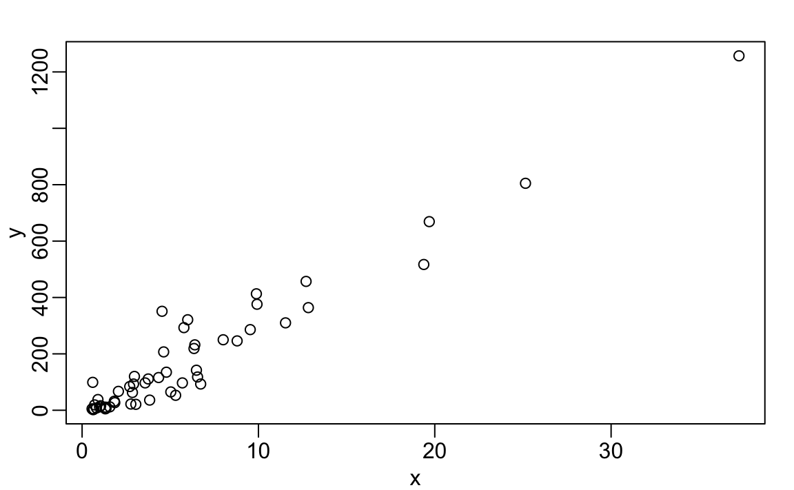
For a quick plot that avoids accessing variables twice, we can apply the with function:
with(murders, plot(population, full)) The part with lets united states of america utilize the murders column names in the plot function. It also works with whatsoever data frames and whatsoever function.
hist
We will depict histograms equally they relate to distributions in the Data Visualization part of the book. Here we will simply annotation that histograms are a powerful graphical summary of a listing of numbers that gives you a general overview of the types of values you accept. We can make a histogram of our murder rates past just typing:
x <- with(murders, total / population * 100000) hist(x) 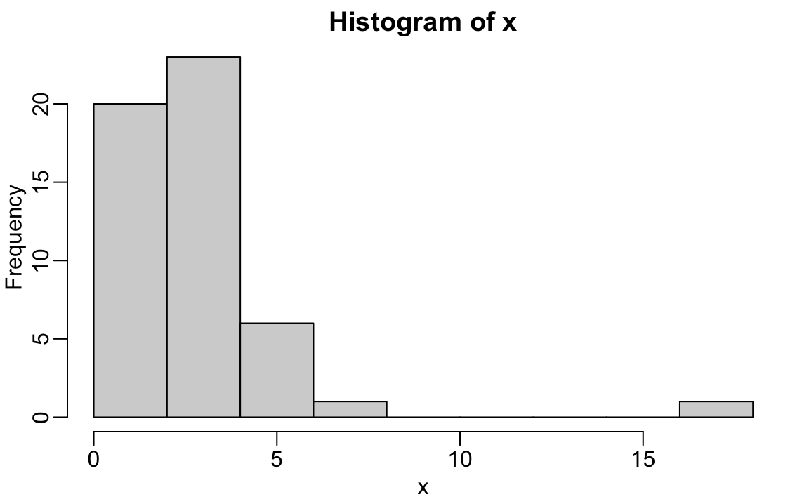
We can see that there is a wide range of values with most of them between 2 and 3 and i very extreme case with a murder rate of more than 15:
murders$state[which.max(x)] #> [1] "District of Columbia" boxplot
Boxplots volition also exist described in the Data Visualization part of the volume. They provide a more terse summary than histograms, merely they are easier to stack with other boxplots. For example, here we can use them to compare the dissimilar regions:
murders$rate <- with(murders, total / population * 100000) boxplot(rate~region, data = murders) 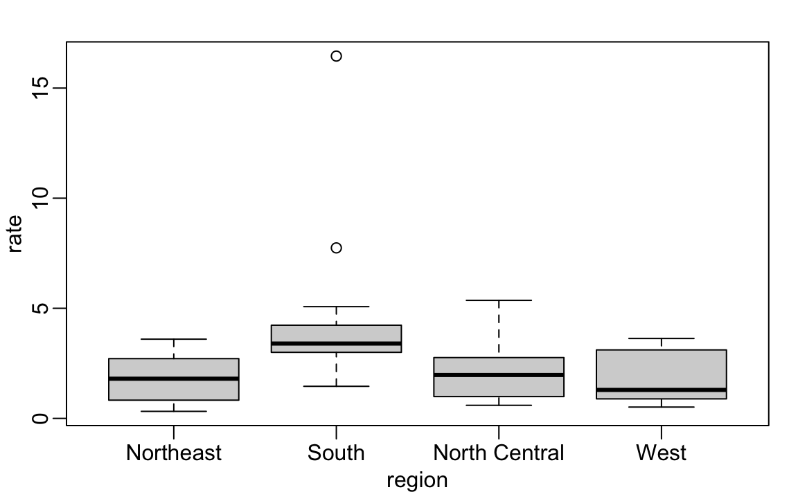
We can see that the South has higher murder rates than the other 3 regions.
image
The paradigm function displays the values in a matrix using color. Here is a quick example:
x <- matrix(1 : 120, 12, 10) epitome(10) 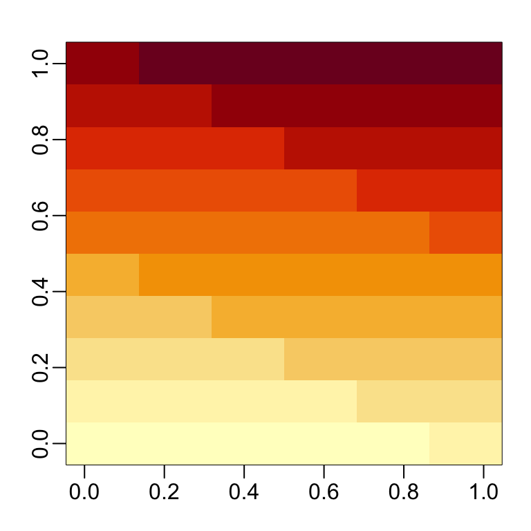
Exercises
1. We made a plot of total murders versus population and noted a strong relationship. Not surprisingly, states with larger populations had more murders.
library(dslabs) data(murders) population_in_millions <- murders$population/ x ^ vi total_gun_murders <- murders$total plot(population_in_millions, total_gun_murders) Go along in mind that many states take populations below 5 million and are bunched upwards. We may gain further insights from making this plot in the log scale. Transform the variables using the log10 transformation so plot them.
2. Create a histogram of the country populations.
3. Generate boxplots of the state populations by region.
Source: https://rafalab.github.io/dsbook/r-basics.html
0 Response to "We Are Again Working With the Characters Abbs C Ma Me Mi Mo Mu"
Post a Comment